FlexFlow

FlexFlow is a deep learning framework that discovers a fast parallelization strategy for distributed DNN training. It uses SOAP (Sample-Operation-Attribute-Parameter) search space of parallelization strategies. in short, FlexFlow automates the parallelization of model training.

The four elements in SOAP search space represent something that can be sliced into smaller chunks. For example, sample and parameter can be thought of as slicing training data and model parameters. Operation describes how operations (e.g. matmul, add, etc.) can be parallelized. Attribute further describes how to partition a sample.

Problem Inputs

Since FlexFlow is about searching for solutions, the framework is given two inputs: an operator graph \(\mathcal{G}\), which include all operations and state in a DNN model, and a device topology \(\mathcal{D}\). Both are described as graphs.

Each node \(o_i \in \mathcal{G}\) is an operation (e.g. matmul). Each edge \(o_i, o_j \in \mathcal{G}\) is a tensor. In contrast, each node \(d_i \in \mathcal{D}\) is a computing device, and edge edge \((d_i, d_j) \in \mathcal{D}\) is hardware connection (e.g. NVLink, network link, etc.), Each edge are also labeled with its bandwidth and latency.

The FlexFlow optimizer uses the operator graph \(\mathcal{G}\) and the device topology graph \(\mathcal{D}\) to generate a discovered strategy to a distributed runtime.

How to search for parallelization strategies

Ultimately, FlexFlow is trying to achieve two things: find parallelization configuration on the operator graph \(\mathcal{G}\), and map the output the device topology \(\mathcal{D}\).

For an operation \(o_i\), it is given parallelizable dimensions \(\mathcal{P}_i\), which is the set of all divisible dimensions in its output tensor. The paper provides a 1D convolution example:

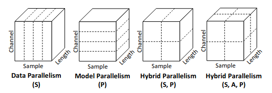
For data parallelism, we can see the input data is splitted into smaller micro-batches. In model parallelism, the batch dimension remains the same, while the model is splitted and handles the same input data. The intuition is for a given tensor, there exists many ways to divide it.

There are many dimensions in \(\mathcal{P}_i\), each single parallelization configuration is denoted as \(c_i\). Therefore, the product of all \(c_i\), represented as \(|c_i|\), is the total number of divided output tensors.

Each parallelization configuration \(c_i\) partitions the operation \(o\) into \(|c_i|\) tasks. (denoted as \(t_{i:1}…, t_{i|c_i|}\)). Each task represents a divided operation and is assigned to a device. The paper claims that, given the output tensor of a task and its operation type, we can infer the input tensors to execute each task. It gives an example of dividing the matmul operation:

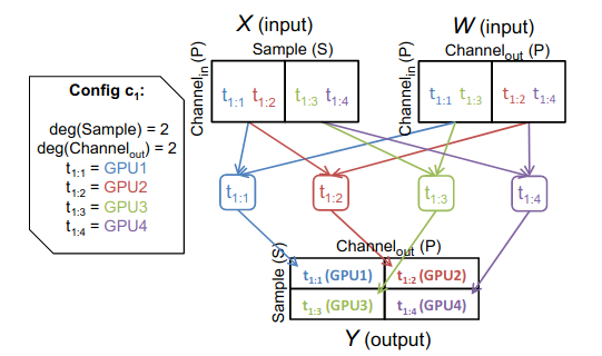
Given the output tensor is splitted across its sample (batch) dimension and feature dimension, and the task type is matmul, we can use these information to infer the input tensors \(X\) and \(W\).

The parallelization configurations \(c_i\) for each operation \(o_i\) is combined in a final configuration \(\mathcal{S}\).

Building Task Graph

Now we have the operation graph \(\mathcal{G}\), the device topology graph \(\mathcal{D}\), and the parallelization strategy \(\mathcal{S}\), we can construct the task graph.

In essence, the task graph specifies the dependencies between each computation and communication task. The task graph is denoted as \(\mathcal{T} = (\mathcal{T}_N , \mathcal{T}_E)\). If two tasks are assigned to the same computation device (e.g. same GPU), no communication task is required. Otherwise, we add a communication task to \(\mathcal{T}_E\). For example, given a operator graph with a set of configurations \(\mathcal{S}\):

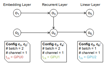
The task graph will reflect the logical dependency between each task:

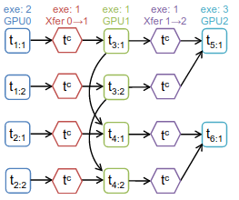
Each computation task is also marked with its average execution time exeTime (from running on the real device multiple times). A communication task’s exeTime is calculated by dividing the tensor size by the bandwidth.

Use Simulation to Estimate Execution Overhead

Now that we have the task graph with all dependencies specified, it’s time to evaluate (or simulate) the execution time of the whole task graph.

In essence, we know how a model is partitioned and placed in a cluster, we need to figure out how to schedule the execution.

The simplest way to simulate the task graph execution is as follows:

• Given a task graph, if there are some task nodes that doesn’t have an input/s, meaning such tasks represent the beginning layers of a neural network, then they are put into a ready queue waiting to be executed.
• Next, we dequeue the task from the ready queue based on the ready time (the time it is enqueued), or the previously executed task’s finish time.
• After this task finishes (simulated) execution, we look at other tasks that depend on this just-finished-execution task, if the other tasks’ dependees all finish execution, then this task can be put into the ready queue.

However, we haven’t seen how the task graph \(\mathcal{T}\) might change once we update the configuration of an operation node \(o_i\). FlexFlow only propose a new parallelization strategy by change the configuration of a single operation \(o_i\) at a time. Therefore, whenever we generate a new configuration for an operator, we only need to re-simulate task involved in the portion of the execution timeline that changes. It means we can generate a new task graph from a previous task graph, thus speeding up the simulation process.

Execution Optimizer

Previously, we assumed the parallelization strategy is generated through some black box function. In fact, the execution optimizer is in charging of taking an operator graph and a device topology as inputs to find an efficient parallelization strategy.

In fact, the optimizer uses Markov chain Monte Carlo (MCMC) method to sample generated parallelization configurations. It uses the simulation cost as an oracle so that the proposed new configuration will be more likely to be sampled from the ones with less simulation overhead. This method is very greedy but the author argue it can potentially escape from local minimum.