Fault Tolerance in Distributed Systems

No systems can provide fault-free guarantees, including distributed systems. However, failures in distributed systems are independent. It means only a subset of processes fail at once. We can exploit this feature and provide some degree of fault tolerance. The problem is, fault tolerance makes everything else much more difficult.

The most common fault models is the fail-stop. It means a process completely “bricks”. When a process fail-stops, no messages can emerge from this process any more. We also don’t know if this process will ever restart. In addition, we must account for all possible states of the faulty process, including unsent messages in the process’s queue. On the other hand, it’s important to point out a process that takes a long time to respond is indistinguishable from a fail-stop. The intuition is such processes and the faulty ones may take an unknown amount of time before message emerge.

We use an example here to illustrate how and why a system fails to provide fault-tolerance. We take a system that replicates data by broadcasting operations using logical timestamps. This system uses Lamport clock to update local clocks (our previous post on Lamport Distributed Mutual Exclusion explains how Lamport clock works). In short, we overwrite the value stored in a replica if an incoming message has later timestamp \(ts\).

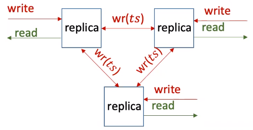
This system is not fault-tolerant. Imagine when one replica receives a write (marked by red incoming “write”) request and then tries to write the value to other replicas. This replica then fail-stops right after it writes to one replica and never writes to the other replica. In this case, not all replicas see the writes, thus violating consistency.

The solution to this problem is quite simple: reliable atomic broadcast. Under atomic broadcast, all writes are all-or-nothing. It eliminates the possibility for a process to fail-stop amid broadcasting.

Now let’s take the above example and update it with additional requirements. Instead of overwriting existing values, we append writes to an array and want to ensure every replica has the same array eventually. The major difference is that replicas needs to wait for acks with higher timestamps before it can append to its array.

This system is also not fault-tolerant. If one replica fail-stops, others will wait forever on a write, because every replicas relies on acks with higher timestamps before committing the append.

Thus, we want to extend the atomic broadcast so that updates become ordered. Under ordered atomic broadcast, writes are all-or-nothing and everyone agrees on the order of updates. If we assume the system to be fully asynchronous, ordered atomic broadcasts are not possible: (1) we can’t guarantee termination under asynchrony; (2) we could lose order. Thus, we rely on the synchronous approach.

Under the synchronous assumption, we can safely say a process fails after waiting for time \(t _{fail}\), where \(t _{fail} = 3 t _{msg} + 2 t _{turn}\). Here, \(t _{msg}\) is the message transfer latency, and \(t _{turn}\) is the max time to respond to a message.

To see why \(t _{fail}\) is calculated this way, we use the following example to explain the process:

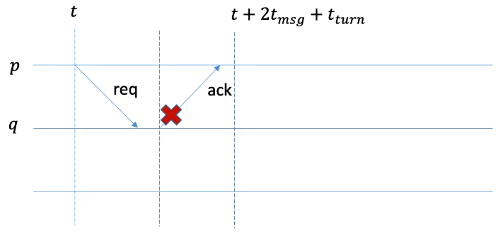
Imagine process \(p\) sends a message to \(q\) and waits for an ack from \(q\). Before \(q\) is able respond with the ack, it somehow crashes. The max time taken for \(p\) to see an aco from \(q\) would be two message transfer time plus the execution time by \(q\), which is \(2t _{msg} + t _{turn}\). We add \(t\) to indicate the elapsed time when \(p\) sends the request.

Now imagine \(q\) is able to broadcast a request right before it fails. Later, another process is able to forward this request back to \(p\). Then \(p\) needs to wait for three message transfer time plus two message processing time before it can assume that it will no longer receive message from \(q\).

Under the synchronous assumption, ordered reliable atomic broadcast works as follows:

• When a client send a request to process \(p\), the process records logical time \(r _l(p,p)\) and physical time \(r _{t}(p,p)\). Then it broadcast the request.
• When process \(p\) receives a message \(m\), and if message \(m\) contains previously unseen timestamp \(t_m\), then we record the logical time we see message \(m\) at \(p\), denoted as \(r_l(p, p_m)\) as well as the physical time \(r _t(p, p_m)\). Then we broadcast the request. Finally, we send an ack back to the originator \(p_m\) without updated timestamp.
• When process \(p\) receives a message \(m\), \(p\) updates \(t _l(p, p_m)\). It means we update \(p\)’s notion of the latest timestamp of another process who just acked.
• Process \(p\) sets another process \(q\) as “failed” (denoted by \(f(p, q)\)) if \(t _l(p, q) \leq r _l(p, p’) < +\infty\) and \(t _t < r _t(p, p’) + t _{fail}\). In short, it means if we broadcast message and don’t receive any response after time \(t _{fail}\), and our last recorded logical time of process \(q\) is before our broadcast, then we know process \(q\) must have failed.
• Then we perform updates when for all \(q \neq p\), \(r _l(p,p) < r _l (p, q)\) (meaning everyone else’s request time is later than mine) and \(t _l(p,q) > r _l(p,p) \lor f(p, q)\). Intuitively, it means we only perform updates when we receive message from other processes after our broadcast, and when we think other processes’ timestamps are after us, or when they have all failed.